Classic Guitar Intonation

by Greg Byers from his 1995 GAL Convention Workshop

One of the first things I noticed when I started playing the guitar as a teenager was that it was frustratingly hard to tune. I really wasn't sure what was going on. It turns out to be a rather intractable problem in a lot of ways.

When I first started building classical guitars in the early '80s John Gilbert told me about his method for setting intonation. At about that time he published an article on the subject in Soundboard.1 I read it, but didn't understand his thought process. Shortly thereafter I ran across an article in the Journal of Guitar Acoustics by Bill and Pat Bartolini.2 They describe a method which involved shortening the fingerboard slightly, as did Gilbert's. I eventually thought I understood the Bartolini article, but I felt they had the details wrong.

I started working on my own theory about ten years ago. I've pondered it over the years, trying to develop a theory that holds water and that could be both useful and understandable. Fortunately, I've recently had some invaluable help from my friend Cem Duruöz, who is a classical guitarist from Turkey, and also a PhD physics student at Stanford. Without his help on the math I could not have completed this project. It's really a collaboration, although any errors are my responsibility.

There is quite a bit of math in what follows, and I'm not expecting you to understand all of it. It's not a simple problem. I'll guide you through my thought process and hopefully we can come out the other end with some practical solutions.

From the very first development of fretted instruments, luthiers have had to consider the questions of temperament and intonation. The question, after all, is "Where do you put the frets?" Vihuelas, lutes, and viols all had movable gut frets on at least most of the fingerboard, which could be tuned by the player. Bermudo in the 16^th century recommended this, but he also apparently complained that they were often tuned by the player with disastrous results.3

He recommended, as did some others of the time, tuning the frets in whole number ratios. Across the top of Table 1 I have given you the fret number (\(n\)) up to 12. DMS means "diatonic major scale," so here I've just given you the letter notes for an E string. Bermudo suggested tuning to Just intonation, which is indicated in the third row. Here \(X_0\) is the total scale length and \(X_n\) is the distance from the \(n^{th}\) fret to the saddle point. For Just intonation these two quantities are in whole number ratios, as are given here. So for the second note of the DMS the distance to the bridge is \(8/9\) the total scale length; the third note distance is \(4/5\), the fourth note distance is \(3/4\), and so on, so that by the time you get up to the octave you are at \(1/2\) the scale length.

This plan worked fine for one course of strings but when you started putting chords together it began to break down. The major reason was that the whole step interval ratio was of more than one size (see Table 1, "interval ratio"). For the first whole step you had an interval ratio of \(8/9\), but for the second whole step you had an interval ratio of \(9/10\). This created problems whenever you tried to change keys or play chords across strings.

At the same time that Bermudo was recommending this, another method was widely used and probably has been around for virtually as long as fretted instruments have been around, and that was to use a constant ratio for succeeding halfsteps. This was undoubtedly discovered empirically and is often called the "Rule of 18." What the luthier did was to make the distance from each succeeding fret to the saddle point \(17/18\) the distance of the previous one (see Table 1, "Rule of 18"). Let's assume we have a scale length of 650mm. The zero fret, or nut, is 650mm from the saddle point. The first fret is \(17/18\) of that distance to the saddle, the second is \(17/18\) of the first fret distance, or \((17/18)^2\) times the total scale length, and so on up to the 12^th fret, where the distance to the saddle would be \((17/18)^{12} \times 650\). If you multiply this out you get 327.4mm. That's not exactly half of 650, but it is fairly close. In fact, it is not bad as an approximation because it provides a built-in method for producing saddle setback. It works better than you might imagine.

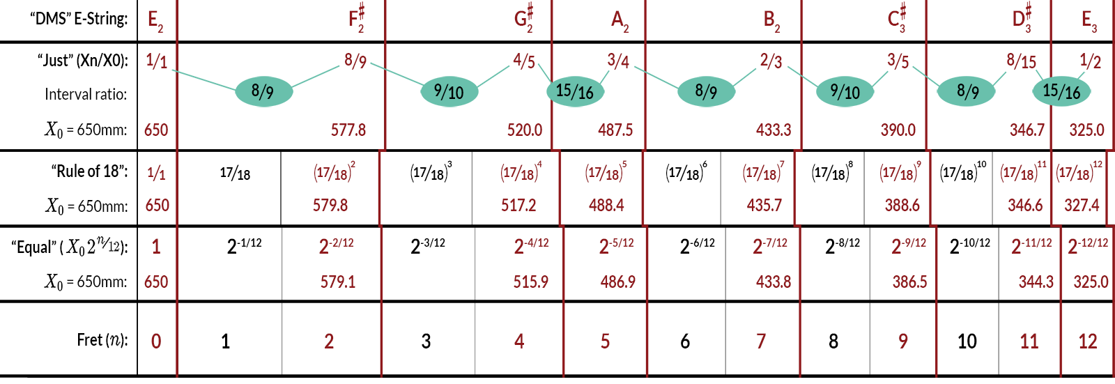
Now let's look at the method we currently use for setting fret placement, which is sometimes called "equal temperament." It is very similar to the Rule of 18 in that the octave is divided into 12 regularly-spaced intervals. The difference is that the 12^th fret is arranged to be at the halfway point. The equation which spells this out is:

$$ X_n = X_0\cdot2^\frac{-n}{12} $$

where \(X_n\) is the distance from the \(n^{th}\) fret to the saddle and \(X_0\) is the distance from the "zero fret," or nut, to the saddle, i.e., \(X_0\) is the total string length. We generally don't distinguish between the distance between nut and saddle (\(X_0\)), and total string length (\(L_0\) in what follows), which, depending on saddle height, is marginally longer. Although the distinction is necessary for the math, there is no practical difference (see Fig. 2).

This equation reads "x sub n equals x sub zero times two to the minus n over twelfth power." You might be familiar with the well-known relation between frequency (f) and the notes (n) of a chromatic scale:

$$ f_n = f_0\cdot2^\frac{n}{12} $$

The frequency of the n^th note of a chromatic scale is equal to the frequency of the first note of the scale times 2 to the \(n/12\) power. Frequency is inversely proportional to string length and from that you can derive Equation 1.4 Observe that the distance between the nut and the first fret under the Rule of 18 is the scale length divided by 18. With equal temperament it is the scale length divided by approximately 17.817.

If you set your frets according to this equation and pay close attention, you will notice the notes get progressively sharp as you go up the scale unless you make some sort of compensation at the saddle. This is why we all move our saddles back away from the nut to some degree. The question then becomes "How far back should we set it?". The answer we often apply is to compare the harmonic at the twelfth fret with the fretted note, and set the saddle so they are in tune. But that's only an approximation. If you play unisons and octaves up and down the fingerboard, you will find that they don't all play in tune even if you get those twelfth-fret harmonics exactly the same as the fretted twelfth-fret notes.

There are a number of reasons for this. One of them, sadly, is that unless strings are uniform in diameter and density throughout their length they will not play in tune. String manufacturers do the best they can, but there will be some variation. This is not something we can compensate for with setup.

Beyond string quality, the major reasons for poor intonation have to do with the fundamental properties of strings. There are two properties of particular importance to us, namely elasticity and inharmonicity. Since both elasticity (stretch) and inharmonicity (stiffness) have tangible effects, any theory about intonation should take both these factors into account.

As we all know, to stretch a string is to increase its pitch. When we fret a note on a guitar we are stretching the string to meet the fret, and that slightly increases the pitch. One of the principal problems that we have to overcome is the fact that open strings do not have this extra stretch, while fretted strings do.

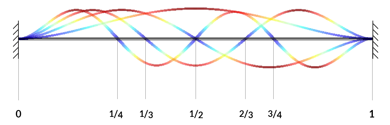
Inharmonicity has to do with the stiffness of the string. All strings have stiffness. The sound of a plucked note consists of the fundamental and an overtone series. An ideal string has a harmonic overtone series, in which each succeeding mode of vibration is a whole number multiple of the fundamental. Fig. 1 depicts the standing waves for each of the first few modes of vibration. It shows that for each succeeding mode the number of nodal points increases by one, and that they are equally spaced along the length of the string. The first mode is the entire string length. For the second there is a node in the very center of the string. At the same time, the string vibrates in thirds, in quarters, and so on.

Ideally, this would give a harmonic series of overtones, but because the string has stiffness, the higher you go in overtone number, the more twists and turns the string must undergo, and the more the stiffness tries to resist that vibration. In the end, that stiffness slightly raises the pitch of succeedingly higher overtones. When we hear a plucked string, our ear/brain mysteriously performs a complicated integration of all these overtones to decide what the perceived pitch should be. Consequently, the note we hear is slightly sharper than the actual fundamental of that note. And as we shorten string length by fretting higher up the fingerboard, both the fundamental and the perceived pitch will be increasingly sharper than we might expect.

I will now present a mathematical model for how this all fits together. What follows is difficult, and probably will not be fully understood even by the mathematically literate on the first few tries. Be not dismayed. Mathematics is just a very careful way of thinking and communicating about a problem. It exposes all your assumptions and understanding in a particularly naked and honest way. It doesn't shift like the quicksand of nuance our words often carry. Very often what we seek from a mathematical theory, in spite of apparent precision, is not an ironclad numerical result, but rather a deeper qualitative understanding that can point to a better practical solution. Such is the case in what follows, where we will explore the implications of string stretch and stiffness for intonation, which will in turn motivate a way to experimentally determine optimum nut and saddle placement.

If you follow a particular method for setting intonation and are happy with the results, skip this article. If upon playing unisons and octaves up and down your fingerboard you find some of them wanting, and you want to know why, try to follow the theory spelled out here, or at least the conclusions drawn. If you want to improve your intonation, check out the experimental results at the end of this article.

The Model — Stretch First

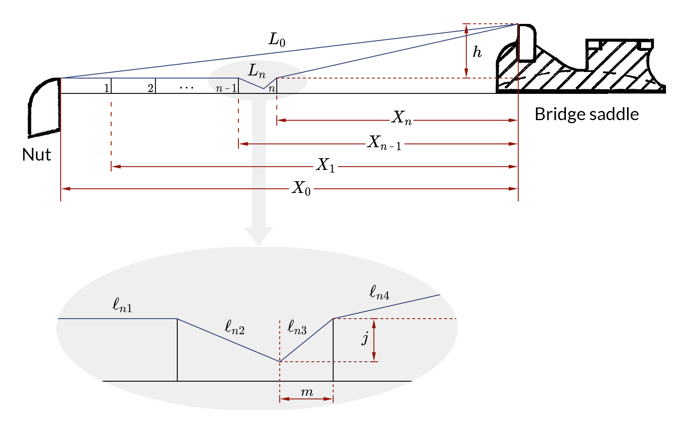
This model treats stiffness and stretch separately. Let's start with stretch. The basic parameters of this part of the model are diagramed in Fig. 2. This follows the Bartolinis' model rather closely, the main differences being notational. It represents an idealized model of what goes on when you fret a note on a guitar. \(X_0\) is the distance between nut and saddle and is the nominal scale length. The distance from the \(n^{th}\) fret to the saddle is \(X_n\), as determined by Equation 1, where n = (1, 2, 3,...). \(L_0\) is the actual length of the open string. Fret positions 1 and 2 are shown, and of course the series could continue as far as you like. Also shown are \(n\), which represents the fret we are choosing to examine, and \(n-1\), which would be the fret immediately behind that fret.

\(L_n\) is the length of the fretted string, which has to go through some deformation and stretching. In the model this is done in an idealized form (see enlarged portion of Fig. 2). We actually fret a note with a finger, not some sort of knife edge, but in order to make the mathematics tractable this model will suffice. We can vary m, the distance from the nth fret that the low point sits; we can change j, the amount you can depress the string. This is just a simple way of introducing the same range of variability produced by a finger.

The fretted string, or \(L_n\), can be broken up into four straight segments. They would be from the nut to the fret behind the fingertip (\(\ell_{n1}\)); from the fret to the fingertip (\(\ell_{n2}\)); from the fingertip to the fret in front of the fingertip (\(\ell_{n3}\)); and from the fret to the saddle (\(\ell_{n4}\)). In what follows, \(\ell_{n4}\), which is the vibrating segment of the fretted string, is going to be referred to as just \(\ell_n\). The sum of these segments is \(L_n\).

We are going to be specifically interested in a couple of quantities which we'll call \(Q_n\). and \(R\) (Fig. 2). \(Q_n\) is defined as the change in string length as a result of fretting (and stretching) it at the n^th fret, divided by the total string length, \(L_0\):

$$ Q_n = \frac{L_n-L_0}{L_0} $$

More generally, for any string length \(L, \; Q=\Delta L/L \), where \(\Delta L\) reads "change in L."

\(R\) is defined as the amount of frequency change relative to the initial frequency that is induced by a given relative change in string length through stretching:

$$ R = \frac{\Delta f/f}{\Delta L/L} $$

\(R\) is a unitless quantity which is going to vary for each of the six strings on your guitar. It will also differ somewhat with different brands and tensions of strings. A little later I will show you how to measure \(R\). I should say here that most of this, including the concept of \(R\) and how to measure it, is due to the Bartolinis. What follows now, however, departs from their work.

Let's examine the mathematics of this geometric model. I mentioned frequency is inversely proportional to string length. More precisely,

$$ f = \frac{1}{2L}\sqrt{\frac{T}{\rho s}} $$

where \(T\) = string tension, \(s\) = cross-sectional area, and rho (\(\rho\)) = density. This works equally well for monofilament strings and for wound strings with a core of nylon floss and wound metal coating. To simplify the notation, let

$$ b(L) = \frac{1}{2}\sqrt{\frac{T}{\rho s}} $$

read "b of L." This simply means b is a function of string length. That is, as L is changed by stretching it, its tension, density, and cross-sectional area are going to change too, to some small degree. Now we can say

$$ f_0 = \frac{1}{L_0} b(L_0) $$

We are looking for the frequency at the n^th fret. We want to allow the fret position to vary such that the frequency fits our standard formula for the note of the scale, that is, find

$$ f_n = \frac{1}{\ell^\prime_n} b(L_n) $$

such that

$$ f_n = f_0\cdot2^\frac{n}{12} $$

This corrected fret position is denoted by \(\ell'_n\) (read "l prime sub n.") We're going to move the fret from its usual position in such a way that we get the right pitch. First of all in order to do this we have to evaluate \(b(L_n)\). That is to say, \(b(L)\) varies depending on which fret you're actually stretching the string to. We use calculus for this (Taylor's theorem), but the details aren't really important. The results are what we need ton pay attention to. We get an equation like this:

$$ f_n = \frac{1}{\ell^\prime_n} b(L_n) + \frac{\partial b(L)}{\partial L} \bigg\rvert_{L_0} $$

The term

$$ \frac{\partial b(L)}{\partial L} \bigg\rvert_{L_0} $$

(read "partial derivative of b with respect to L evaluated at Lo") expresses how b changes with changes in string length (at pitch) near L = Lo. It turns out that we can relate \(\frac{\partial b(L)}{\partial L} \bigg\rvert_{L_0}\) to \(R\). This is useful because \(R\), as I have mentioned, is a quantity we can measure. Remember from Fig. 2 that \(R\) is defined in terms of frequency change (M) as it relates to string length. Therefore, we need to find out how \(f\) changes with \(b\), i.e.,

$$ \frac{\partial f(b)}{\partial b} $$

Then we can find \(R\) in terms of \(b\) instead of \(f\). After a bit more calculus (again Taylor's theorem) we find that

$$ R = \frac{L_0}{b} \frac{\partial b(L)}{\partial L} \bigg\rvert_{L_0} -1 $$

and consequently

$$ \frac{\partial b(L)}{\partial L} \bigg\rvert_{L_0} = \frac{b(L_0)}{L_0}(1+R) $$

Substituting into Equation 5 gives:

$$ f_n = \frac{1}{\ell^\prime_n} \left(b(L_0) + \frac{b(L_0)}{L_0}(1+R)(L_n-L_0)\right) $$

Don't worry if you're not following the details at this point. Suffice it to say that if you express Equation 2 in terms of \(\ell_n\) and \(b(L)\), and equate Equation 2 and Equation 6, you can solve for \(\ell'_n\):

$$ \ell^\prime_n = \ell_n (1+Q_n(1+R)) $$

The geometry is such that Equation 7 can be expressed with virtually the same precision in terms of \(X\) (fret placement):

$$ X^\prime_n = X_n (1+Q_n(1+R)) $$$$ \;\\ where\\ \;\\ X_n = X_0\cdot2^\frac{-n}{12}\\ \;\\ Q_n=\frac{L_n-L_0}{L_0}\\ \;\\ R=\frac{\Delta f/f}{\Delta L/L} $$

Once we decide on a scale length (\(X_0\)) we can easily evaluate \(X_n\). We know what \(Q_n\) is by evaluating these various string lengths according to our geometric model, and we can determine \(R\) experimentally.

Experimental Interlude: Measurement of \(R\)

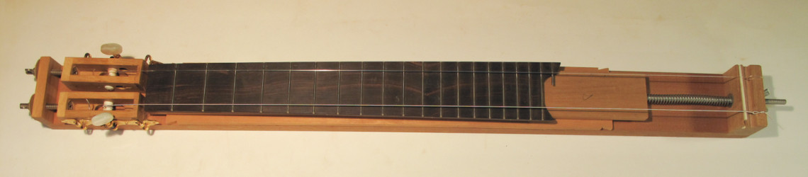
I want to take a moment now to show you how that is done. In their paper, the Bartolinis describe a device for measuring \(R\) similar to the one shown in Photo 1. Recall that \(R\) relates pitch change to string stretch. This device has a tuning machine (in this case two) mounted to a \(1/4 \times 20\) threaded rod, regulated by a wing nut. A scale dividing the circle into tenths behind the wing nut allows you to measure string stretch to within about \({1/200}''\). With this device you can measure a scale length, tune a string to pitch, and then stretch the string with the wingnut and measure the change in pitch that results from a particular amount of stretch. It's a rather crude device really but it gets the job done. For each string you can actually measure the value of \(R\).

The Bartolinis did this for a number of brands of strings. They concluded that for a G string, \(R\) is about 35 and all the other strings are pretty close to one another at about 26. These are dimensionless values. I have made the same measurements on a number of strings and I have gotten values somewhat smaller than theirs (Table 2). My method is slightly different, and I don't know which is more accurate. This is one area where more work needs to be done.

$$ \begin{array}{c|cccccc} \text{string} & E_2 & A_2 & D_3 & G_3 & B_3 & E_4 \\ \hline R & 25 & 23 & 22 & 30 & 24 & 21 \\ \end{array} $$

Results are not as reproducible as one might hope, so for each string you have to make repeated measurements. For every set of strings you're going to get a different set of values, so not only do you have to measure each string repeatedly, but different samples of the same string from the same manufacturer will give slightly different values. Of course, the strings must be prestretched for a while before they will give consistent measurements.

I turned the wing nut until I had increased the pitch by one semitone, as measured with a Seiko chromatic autotuner. I measured how many turns that was, 1.3 or whatever, which represented how much the string had been increased in length. Then I turned it back down to the original pitch and measured that. It's difficult to get a really precise measurement. These numbers I've given you here are averaged for a combination of D'Addario J46 and Augustine Regals with blue label basses, and a few other things. I also measured Savarez Alliance, and those numbers are smaller by about 10% than the numbers I'm giving you here.

Back to the model

Now that we have a value for \(R\) associated with each string, we can, for each string, evaluate Equation 8 and obtain a set of stretch-accomodated fret positions, \(\{X'_n\}\), for the whole scale. As noted previously, this requires, in addition to our experimentally determined values of \(R\), a nominal scale length \(X_0\), and an evaluation of \(Q_n\). This is determined just by cranking the numbers on our geometric model for a particular saddle height, fret height, and so on.

Because the parameters differ, we get a different set of fret positions for each string. That doesn't do much good if we want to set properly-placed frets for all strings at once. Somehow we've got to figure out a way of setting the frets to work across all strings even though each set of \(\{X'_n\}\) is different. The way we do it is to fit each of our sets of \(X'_n \ast\) to an equation of the form:

$$ X'_n = a\cdot2^\frac{-n}{12} + b $$

* Recall that the subscript n is defined for frets (n=1, 2, 3, ...) but not for the nut position. Even if we allow \(n=0\), Equation 8 will collapse to \(X'_0 = X_0 \), corresponding to the trivial fact that playing the open string doesn't require changing the nut position to stay in tune. Thus, the set \(\{X'_n\}\) does not contain \(X'_0\).

To emphasize its generality, we shall henceforth call this our canonical equation for fret placement. Notice this is identical to our Equation 1, with a equal to \(X_0\) and \(b\) equal to zero. The \(a\), then, in this equation represents scale length. If you make this fit using a curve-fitting statistical package on your computer, you will find that for each string the fitted equation gives a different value of \(a\), which I call \(X''_0\). (read "X double prime sub 0"). This, then, is a new scale length. The \(b\) in Equation 9 I call \(\Delta S\), or saddle setback (Equation 10). If you think about it I think you can see why. For each fret position you have to add a little bit more, the same amount more each time. That's what \(b\) is, and that's what saddle setback is:

$$ X'_n \approx X''_0 \cdot 2^\frac{-n}{12} + \Delta s\\ \;\\ \approx X''_n + \Delta s $$

Once we do this we can also calculate a nut position. Think about it this way. When we derive this set of fret placements \(\{X'_n\}\), we find in each instance we have to set the fret slightly farther back toward the nut from its initial position. The model does this to increase the fretted string length to compensate for the increase in pitch that results from stretching the string. It does this for every fret except the zero fret (i.e., the nut) because in this case the string is unstretched (unfretted). This results in a relative shift in nut position, \(\Delta N\). Mathematically, this is expressed as:

$$ \Delta N = X_0 - (X''_0 + \Delta S) $$

Since (\(X''_0 + \Delta S \)), which comes from our canonical approximation to \(\{X'_n\}\) (Equation 10), is larger than \(X_0\), \(\Delta N\) is a negative number. I define it this way to emphasize the fact that, in practice, \(\Delta N\) is subtracted from the end of the fingerboard, shortens the distance between the nut and the frets, and indeed, shortens the total length of the string.

Now we have newly calculated fret positions, \(X''_n\) that follow our canonical formula (Equation 10); we have saddle setback, \(\Delta S\); and we have found a new nut position, \(\Delta N\). We end up with a set of fret positions that, as it turns out, are very close to the theoretical values from our model for string stretch, \(X'_n\). Each string has a different set of values but because \(X''_n\) is in canonical form, we can scale each \(X''_0\) up to, let's say, 650mm, so that there is a common nominal scale length for each string. This allows us to cut our fret slots in the normal way for all strings and just make appropriate adjustments at the nut and saddle.

This may sound like slight of hand but it's quite important to try to understand. Our model leaves \(L_0\) (or \(X_0\)) fixed as we calculate fret positions to accommodate string stretch. Even our fitted equation is consistent with this fact, as we see if we rearrange Equation 11:

$$ X_0 = X''_0 + \Delta S + \Delta N $$

What we want, however, is to lift this constraint and scale this equation so that, instead, \(X''_0\) is constrained to be equal to some chosen nominal scale length. This permits us to cut the same fret slots for all strings.

The Model — Adding Stiffness

Now I'd like to briefly go through the stiffness part of the model. Stiffness is easier to say than inharmonicity, and because it suggests an intuitive aspect of the concept, perhaps it is just as well to use this term. Recall that in an ideal string you have a harmonic series of overtones or partials, but in a real string each partial gets successively sharper, the higher you go. Equation 135 is the governing equation for this phenomenon:

$$ v_p =\frac{p}{2L} \sqrt{\frac{T}{\rho s}}\left( 1 + \frac{2}{L}\sqrt{\frac{Es\kappa^2}{T}} + (4 + \frac{p^2\pi^2}{2}) \frac{Es\kappa^2}{TL^2} \right) $$

Here, \(v_p\) (read nu sub p) is the actual pitch of the partial in question. For example, the fundamental is represented by \(p = 1\). \(E\) is the modulus of elasticity, which is a property of the material the strings are made of, how much it stretches for a given tension. Two other properties of the string are represented by \(s\), the string's cross-sectional area, and kappa (\(\kappa\)), which is a quantity called the radius of gyration. This is a property of the geometry of the string, and for an unwound string kappa equals \(r/2\), where \(r\) is the radius of the string.

It will help to simplify the notation a little. Let

$$ \alpha = 4 + \frac{p^2\pi^2}{2} \quad and \quad \beta = \sqrt{\frac{E s \kappa^2}{T}} $$

Now for the fundamental we have:

$$ v_1 =\frac{1}{2L} \sqrt{\frac{T}{\rho s}}\left( 1 + \frac{2\beta}{L} + \alpha\frac{\beta^2}{L^2} \right) $$

The terms within parentheses in this equation account for the stiffness of the string.

Audience: Is the string fixed at nut and saddle or does it ride over nut and saddle?

I'm not sure how that changes things but that's a fair question. For inharmonicity it is assumed to be fixed at nut and saddle. For the calculation of \(R\) the string rides over the nut and saddle. I didn't investigate the case where it is fixed but I assume the difference would be subtle.

So what do we do with this? As I mentioned, vi is the frequency of the first partial, and in the case where we let \(L\) be the total string length, it serves as a good approximation to the perceived pitch of the open string. So we can look at the frequency of the open string and compare that to the frequency of the fretted string. We are going to keep it simple and just look at the frequency of the fundamental and use that as an approximation for the perceived pitch even though that flies in the face of what I said earlier. Just looking at stiffness, not stretch, we see that what really changes here is \(L\). So, again, what we want to do is write an equation for the frequency of the fretted note, allowing for adjustments (\(\Delta \ell_n\)) in the placement of the frets to keep the fretted notes on pitch:

$$ f_n =\frac{1}{2\ell'_n} \sqrt{\frac{T}{\rho s}}\left( 1 + \frac{2\beta}{\ell'_n} + \alpha\frac{\beta^2}{{\ell'_n}^2} \right),\\ \;\\ where \\ \;\\ \ell'_n = \ell + \Delta \ell_n $$

Then we solve for \(\ell'_n\), keeping in mind that \(\ell_n\) and \(L_0\) are defined as in our original geometric model. I'm not going to go into detail like I did with stretch, but if you work through the math you eventually end up with:

$$ \ell'_n = \ell_n \left(1 + \frac{2\beta}{\ell_n} - \frac{2\beta}{L_0} + \frac{\beta^2}{\ell_n^2}(\alpha -8) - \frac{\beta^2}{L_0^2}(\alpha -8) \right) $$

Now we can combine both parts of the model. It turns out they combine multiplicatively, indicating they are not completely independent in their effects:

$$ \ell'_n = \ell_n \left( 1 + Q_n(1 + R) \right) \left( 1 + \frac{2\beta}{\ell_n} - \frac{2\beta}{L_0} + \frac{\beta^2}{\ell_n^2}(\alpha -8) - \frac{\beta^2}{L_0^2}(\alpha -8) \right)\\ \;\\ or: \\ \;\\ \ell'_n = \ell_n \times stretch \times stiffness $$

It looks complicated. Indeed, it was even more complicated before we dropped the higher-order terms. But take heart: all of these things can be evaluated. DuPont will give you a number for the modulus of elasticity of the nylon used, and you can measure directly the density, the cross-sectional area, the tension, the string length, and the radius of gyration. So we can actually calculate \(\ell'_n\).

There are a number of things we can learn from this model. In Tables 3 and 4 I have given some computer-generated results for just the stretch portion of the model. We have calculated \(\{X'_n\}\) for each string, using appropriate values of \(h\), \(R\), \(M\), and \(j\). We have then fitted these theoretically-derived points to our canonical equation (Equation 9) and from that we've been able to calculate what the saddle and nut positions should be.

In Table 3 I've set \(j = 0.3mm \). I'm assuming my frets are about a millimeter high, so with \(j = 0.3\) that triangular string deformation in Figure 2 goes about a third of the way down to the fingerboard. I've also assumed that \(j\) decreases as you go up the fingerboard. That is, when you press behind the first fret, your finger goes farther toward the fingerboard than it would at the twelfth fret. I've modeled this as \(j = 0.3(X_n/X_1) \). Thus, for the first fret \(j = 0.3\), and for the twelfth fret \(j\) equals roughly half that amount. In Table 4 I've set \(j = 0.5mm\), assuming that you're pressing your finger a little more solidly into the string. I've done this to see how sensitive the model is to the value of \(j\). Frankly, this is one of the problems we have, that different players have different touch. We need to find out what kind of difference that's going to make.

Let's take a look at the numbers in Tables 3 and 4. Saddle setback is in the neighborhood of 0.5mm to a little over 1.0mm. In Table 3, where \(j\) equals 0.3, the nut is set forward up to 0.25mm. In Table 4, as you increase the amount you press down on the string, the nut can move forward as much as 0.5mm. So we see that nut placement is sensitive to how hard you press the strings. Imagine you're fretting at the first fret. The more you press, the more you're going to stretch that string, and the sharper you are going to be relative to the open string.

For now this is all I want to comment on except to point out the column on the right labeled \(\chi^2 \) (Chi squared.) This is a measure of how well the numbers fit. The closer \(\chi^2 \) is to zero, the better the fit. In our case, a value of around 0.2 would constitute a poor fit. Remember, we are trying to fit our data points to our equation in canonical form, which allows us to use standard fret placement, and allows us to calculate a saddle setback and a nut "setforth." If it's not a good fit it doesn't do us any good, but these values indicate it's a very good fit. Calculate the value of \(X''_n + \Delta S \) for any fret (\(n\)) you chose and compare it to the theoretical value for \(X'_n \). You will see that they are really close, much closer than you could measurably differentiate.

Now let's look at some results from our attempt to model inharmonicity (stiffness). As I say, this is work in progress, but we can still learn from it. In the case of stiffness only (Table 5), we get considerable saddle setback for the unwound strings, and quite a considerable saddle setback for the G string — almost 4mm. The nut placement, however, remains unaffected. By the way, these numbers are given in hundredths of a millimeter, but actually I find I can't effect a controlled change of less than roughly 0.1mm when I'm setting up a guitar. Further, it's quite unlikely that you could hear a difference of much less than 0.1MM. For these reasons the second digit past the decimal point in these tables is fairly meaningless from a practical standpoint. You can feel free to round up.

Now notice the wound strings. The numbers for saddle change are rather low, indicating these strings are not as stiff. This is not surprising. One of the main reasons bass strings are wound is to reduce their inharmonicity. In addition, the diameters would have to be very large if they weren't wound. So you increase the mass of the string (that's our rho, or density) by wrapping them with windings. In addition, you can see that, relative to stretch, stiffness seems to have more of an effect on saddle setback. Although we shouldn't put too much stock in comparisons between Table 4 and Table 5 because they depend on the parameter values chosen, we see that the wound strings are about equally affected by stiffness and stretch, but on the unwound strings stiffness really takes over in determining saddle setback. Nut setforth, however, is determined only by the stretch. Again, \(\chi^2\) values in Table 5 are extremely small for the stiffness part of the model. In fact they signify a virtually perfect fit.

What happens when you combine the two halves together is depicted in Table 6. I set \(j=0.5\), decreasing in value toward the high frets, and got numbers that look like this: saddle setback is almost 5mm (this is the G string, which is the worst offender), nut setforth is a little over 0.5mm. All right, so that's what the model tells you to do with a few values that I've plugged in. The take-home message is not in the numbers but in the relationships: saddle setback is mostly, but not entirely, neccessitated by stiffness (inharmonicity), and nut setforth results entirely from stretch (elasticity); and on both accounts the G string is the worst offender.

$$ \begin{array}{c|c|c|c|c} \text{string} & X''_0 & \Delta S & \Delta N & \chi^2 \\ \hline E_4 & 649.60 & 0.54 & -0.14 & 0.002 \\ \hline B_3 & 649.42 & 0.73 & -0.15 & 0.002 \\ \hline G_3 & 649.13 & 1.07 & -0.20 & 0.003 \\ \hline D_3 & 649.22 & 0.92 & -0.14 & 0.002 \\ \hline A_2 & 649.05 & 1.10 & -0.15 & 0.002 \\ \hline E_2 & 648.91 & 1.36 & -0.27 & 0.002 \\ \end{array} $$$$ \begin{array}{c|c|c|c|c} \text{string} & X''_0 & \Delta S & \Delta N & \chi^2 \\ \hline E_4 & 649.98 & 0.41 & -0.39 & 0.01 \\ \hline B_3 & 649.85 & 0.59 & -0.44 & 0.02 \\ \hline G_3 & 649.66 & 0.89 & -0.55 & 0.02 \\ \hline D_3 & 649.62 & 0.79 & -0.41 & 0.01 \\ \hline A_2 & 649.46 & 0.97 & -0.43 & 0.01 \\ \hline E_2 & 649.24 & 1.21 & -0.45 & 0.02 \\ \end{array} $$$$ \begin{array}{c|c|c|c|c} \text{string} & X''_0 & \Delta S & \Delta N & \chi^2 \\ \hline E_4 & 648.36 & 1.64 & 0 & 9.25\times 10^{-8} \\ \hline B_3 & 647.29 & 2.71 & 0 & 1.36\times 10^{-7} \\ \hline G_3 & 646.01 & 3.99 & 0 & 5.73\times 10^{-7} \\ \hline D_3 & 649.02 & 0.98 & 0 & 5.73\times 10^{-7} \\ \hline A_2 & 649.17 & 0.83 & 0 & 6.90\times 10^{-7} \\ \hline E_2 & 649.30 & 0.70 & 0 & 8.38\times 10^{-7} \\ \end{array} $$$$ \begin{array}{c|c|c|c|c} \text{string} & X''_0 & \Delta S & \Delta N & \chi^2 \\ \hline E_4 & 648.33 & 2.06 & -0.39 & 0.01 \\ \hline B_3 & 647.14 & 3.30 & -0.44 & 0.02 \\ \hline G_3 & 645.65 & 4.89 & -0.54 & 0.03 \\ \hline D_3 & 648.64 & 1.77 & -0.41 & 0.01 \\ \hline A_2 & 648.62 & 1.80 & -0.42 & 0.01 \\ \hline E_2 & 648.54 & 1.91 & -0.45 & 0.02 \\ \end{array} $$

Experimentation and Results

It wasn't until I had done most of the modeling that I realized there's a simple way to pretty much duplicate my efforts with real strings using the same device I used for measuring \(R\) (Photo 2). I made myself a little section of movable fingerboard to slip under the strings. In the interests of economy the intervals between these frets are such that each piece of fretwire can serve as two different frets (well, almost). Depending on where it is placed along the string length, the highest pair of frets has the same interval as the 16^th and 17^th frets would on a 650mm scale, the next pair has the same interval as the 11^th and 12^th frets, the next has the same interval as the 6^th and 7^th frets, and the final pair has the same interval as the second and third frets. This last one can also serve as a first fret. With appropriate shims under the saddle, you can set saddle height, or \(h\), to any value you want.

To obtain the data in Table 7, I first clamped the device to my workbench. Then I set h to the value I would expect to have for a particular string, given the way I normally set up a guitar. From the top of the twelfth fret to the bottom of the G string is normally about 3.5mm, so if I set \(h\) at the saddle to 7mm I'm going to simulate that. In practice, I set h by just the same procedure as on a real guitar, after first placing the appropriate fret of my movable fingerboard at the 12^th fret position. Now you are ready to actually measure where your frets ought to be placed (\(X'_n\)), provided you have accurately set the distance between nut and saddle to your desired scale length. Tune the string to pitch, depress the string at roughly the 12^th fret position, and pluck the fretted note repeatedly as you move the fingerboard back and forth until it is exactly on pitch. Use the best tuner you can find to determine the right pitch for whichever note you're looking at. With my little fingerboard gizmo I can get experimental values for the 1^st, 3^rd, 7^th, 12^th, and 17^th frets. You could easily use an entire fingerboard cut well short at the nut end to obtain data for all the frets.

Once you've established where the fret position is, you have to measure it very accurately. I used two 500mm steel rules and a hand lens to measure scale length. You can use either nut or saddle as a point of reference, but the measurements must give exactly the same results from either end. It sounds simple but in reality it is painstaking work. You have to do endless repetitions before you get the feeling that by taking averages you may come close to getting a picture of what's really going on.

I went through this procedure with a set of D'Addario strings. When I switched the string end for end, I got different values (laughter). This was true with both plain and wound strings. I was surprised, because I've generally felt that D'Addario J46s have been pretty true. I then tried a set of Augustine Regals with blue label basses. When I switched the strings around they didn't vary as much. The data in Table 7 are from Augustine Regals.

$$ \begin{array}{c|c|c|c|c} \text{string} & X''_0 & \Delta S & \Delta N & \chi^2 \\ \hline E_4 & 649.02 & 1.28 & -0.30 & 0.11 \\ \hline B_3 & 648.59 & 2.14 & -0.73 & 0.08 \\ \hline G_3 & 647.83 & 3.14 & -0.97 & 0.26 \\ \hline D_3 & 649.06 & 1.47 & -0.53 & 0.04 \\ \hline A_2 & 648.72 & 1.73 & -0.45 & 0.01 \\ \hline E_2 & 647.54 & 2.91 & -0.45 & 0.06 \\ \end{array} $$

Remember, with the experimental work I don't have the 19 or 20 data points that we used to calculate the theoretical results. In this case all I've got are average values for frets 1, 3, 7, 12, and 17. That makes five data points. If we had more we could probably fit our equation more precisely, but even with just those five we can indeed fit them to our canonical equation, get a value for \(X''_0\), and then establish what our saddle setback and nut setforth should be. If you look at the \(\chi^2\) values you'll see they're not quite as tight as they were with the theoretical results. This is to be expected because experiments are often messy. All kinds of problems crop up. Just reading the ruler is a major source of error. Even so, it turns out that the \(\chi^2\) values are still pretty good.

Consult Tables 6 and 7 to compare these experimental results with our model for stretch plus stiffness. Remember, when we make the measurements with real strings we are combining both these things. Look at the \(\Delta S\) and \(\Delta N\) columns in both tables. The numbers are not the same but they are of similar magnitude. Both the model and the experimental apparatus can be improved. For instance, the movable fretboard could be mounted on a threaded rod so its position could be more carefully measured. But this similarity of magnitude, I believe, helps validate the principles of the model. There is nothing theoretical about the experimental results, and they are the ones to be applied toward a practical solution.

I think you will find that the way that I'm going to recommend setting up nut and saddle positions will help you accommodate pretty well whichever strings you use. You might have a problem, however, if the player experiments with different kinds of strings, particularly if they use Savarez Alliance and then switch back to something else. That is a fairly big change, and you might have some perceptible intonation problems.

Table 8 shows the last numbers I'm going to throw at you, so take a deep breath! This shows only the G string. Column A shows fret placement, calculated according to Equation 1. Column B is \(X'_n\). These are the numbers that I got using my little gizmo and making the measurements. Column C, \(X''_n + \Delta S\), is the value that I get that's analogous to these, but for the fitted equation. How good a fit is it? We can see by subtracting column C from B. For the 1st fret we are about 0.1mm off; for the 3^rd fret, 0.03mm. For the 7^th fret we're 0.4mm off, which is more than I'd like to see. For the 12^th fret we're off about 0.25mm, again more than I would like to see; and for the 17^th, only 0.02mm.

$$ \boxed{ \begin{array}{c|c|c} & A & B & C & & &\\ n & X_n & X'_n & X''_n+\Delta S & B-C & B-A & B-(A+2.33) \\ \hline 1 & 613.52 & 614.73 & 614.61 & +0.12 & +1.21 & -1.12 \\ \hline 3 & 546.58 & 547.93 & 547.90 & +0.03 & +1.35 & -0.98 \\ \hline 7 & 433.82 & 435.10 & 435.51 & -0.41 & +1.28 & -1.05 \\ \hline 12 & 325.00 & 327.33 & 327.06 & +0.27 & +2.33 & 0.00 \\ \hline 17 & 243.47 & 245.78 & 245.80 & -0.02 & +2.31 & -0.02 \\ \end{array}} $$

An interesting thing is that this doesn't vary in a regular way. In the first two cases my experimentally measured fret positions are farther back than the fitted curve gave them. In the case of the 7th fret, it was farther forward, then back again and forward. I'm hopeful that experimental error is the cause of these fluctuations.

But still, let's compare this to the fit between our experimentally determined fret placements and the standard way of doing business, that is, with no nut adjustment at all. That is, let's compare the congruence between column B and C with the congruence between columns B and A. If you compare the experimentally determined fret positions (column B), with calculated positions using the basic formula (column A), you get values (B - A), which, not surprisingly, are positive and fairly high. This reflects the fact that we have to move the saddle back to get anything like a decent fit. The typical way of determining saddle setback is to play the 12^th fret harmonic and set the saddle so the fretted octave matches that. The harmonic is a convenient substitute for an electronic tuner. From this perspective, then, the typical saddle setback one would calculate with the nut remaining in the standard position is the 12^th fret value of (B - A). When we use that value and then compare to column B, (B - (A + 2.33)), you can see the fit is still not nearly as good as with our fitted equation. Here the fit is very good for the upper frets but very bad (about a millimeter off) for the lower frets. Clearly, our fitted equation, which accommodates moving the nut forward as well as moving the saddle back, is a much better fit to our data. Even if, rather than taking the 12^th fret value for saddle setback, you took an average of all 5 frets for which we have data (giving B - (A + 1.70) for the last column heading of Table 8), you will find the fit is no better. Column C is by definition a mathematically optimum fit to our experimentally derived data. That's really the point of this whole talk, that you can get a much better fit to ideal fret placement by moving the nut and the saddle both, rather than just the saddle.

So how do we go about utilizing these data? First, set your frets according to the standard equation for, let's say, a 650mm scale length. The values we generated for both saddle and nut change are not, however, based on a 650mm scale length, but rather on the value of \(X''_0\), which varies from string to string. For each string it is slightly less than 650 (Table 7), so for each you will need to scale up the magnitude of AS and AN accordingly. This is really little more than a formality since you will find they change negligibly. For instance, for the worst case G string,

$$ \Delta S_{650} =3.14 \times 650/647.83=3.15 $$

When you set your saddle position you cannot distinguish between 3.14 and 3.15mm. So the values presented in Table 7 are my recommendation for Augustine Regals. Further, I believe these data are fairly representative of a broad spectrum of strings and probably are good average values. I haven't done the tests to truly demonstrate this assertion, so you can either try this out or test your own strings and report back to the rest of us.

Jim Loewenherz: For the high E string you have \(X''_0\) o equals 649.02mm. Is that the new, actual string length?

No. I maybe didn't explain this well enough; but this fitted equation, which has \(X''_0\), and also includes \(\Delta S\), and from which we can calculate \(\Delta N\), all of these numbers are for a nominal scale length of 649.02 in the case of that E string. In order to use our standard fret placement we need to scale everything back up from our nominal scale length of 649.02 to 650. But when we do that, because it's so close to 650, from a practical point of view \(\Delta S\) and \(\Delta N\) are still the same. They don't change enough to worry about.

Jim Loewenherz: So on this high E string the actual length of the string from the compensated nut to the compensated saddle would be...?

The actual string length is given by Equation 12 and comes to 650mm. After we scale up to the nominal scale length of 650mm, the string length becomes 650 plus 1.28 (i.e., \(\Delta S\)), or lets just say 1.3, plus -0.3 (i.e., \(\Delta N\)). So the total length from nut to saddle would be 650.9mm.

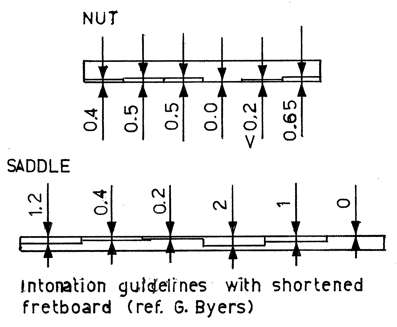
Fig. 3 illustrates how I recommend you shape your nut and saddle to fit these numbers. Roughly speaking, what I do is cut the fingerboard short enough at the nut end so that the most offensive string, which is the G string, is accommodated by setting the nut right up to the end of the shortened fingerboard. In other words, shorten the board by \(\Delta N\), or about 1.0mm. Then for the other strings you can just put a facet on the front face of the nut to move the break point farther back. Measure out these points with a hand lens. Again, let me emphasize that if you can get them to within a tenth of a millimeter of the intended values you are doing well.

Once you have set the nut according to the data, you could do the same with the saddle. However, I recommend setting the saddle facets only approximately and perhaps a little conservatively at first. Then you can use the standard method for establishing saddle setback, playing the fretted note at the 12^th fret and comparing that to the harmonic. It's the simplest way to do it, and it also lets you accommodate to some degree the different kinds of strings you may use.

Tim McCoy: Greg, before you did the mathematical analysis were you doing nut and saddle compensation?

Yes. I thought that conceptually the Bartolinis reall did something neat with their geometric model and witl the concept of \(R\). I also knew what John Gilbert was doing. I wanted to improve upon that, so I started by doing seat-of-the-pants guesstimates of where I though the nut and saddle ought to be. What I've done for a number of years is to cut the fingerboard about 0.5MM short and then facet the nut so that the high E string and the D string both go back almost to the original nui position. The G string is left unfaceted and the others are placed in intermediate positions. Then I set the saddle setback according to the 12^th-fret harmonic. It has been an improved system. Players consistently tell me that my guitars are more in tune than most guitars are. But I have never been fully satisfied with that solution, and I've learned just in doing this analysis that I really was not doing enough compensation at the nut.

Richard Brune: Eugene Clark was working on a very similar concept in the early '60s, just empirically. I don't think he was using mathematics.

Fritz Mueller: Greg, how does your system compare with the one John Gilbert proposed?

Here is what John Gilbert recommended in his 1984 Soundboard article, and what he tells me he still does today. For comparison I have converted his numbers to metric and scaled them so that the fingerboard is slottec according to a nominal length of 650mm. Note that all strings are treated the same.

First, set your nut and saddle to give a Total String Length (TSL) of 649.606mm, as if you used a fingerboard cut to a Basic String Length (BSL) of 648.345mm, with an additional saddle setback of 1.261mm. Hypothetically, the 12^th fret would be 325.434mm from the saddle. But instead of using such a fingerboard, cut your fret slots to a BSL of 650.000mm from which you will then remove 0.827mm from the nut end. Notice that the 12^th fret is still in the same position as in the hypothetical case.

Gilbert's \(\Delta N\), therefore, is -0.827mm. To compare his \(\Delta S\) to mine as I have defined it, it is necessary to use the fingerboard with a BSL of 650mm as a frame of reference. The distance from the 12^th fret to the saddle is 325.434mm, so AS is 0.434mm. If you ask him what his saddle setback is, he will say 0.050", which is equivalent to 1.261mm (scaled appropriately), but as I have tried to show, that figure is not analagous to my \(\Delta S\).

Kenny Hill: I've tried a system more like John Gilbert's. I found that I could adjust to it just fine, but when I played the Steve Reich piece I was out of tune with all the other guitars. (Laughter) It didn't sound real clean playing wit) all these supposedly-out-of-tune guitars.
Richard McClish: The top of the guitar is a resonator in various ways. It's got Q. In a situation where we don't have the apparatus clamped to a granite slab, you'll find that the string behaves as if it ends somewhere other than where-it actually goes over the bridge. This is because of Q. If you have a guitar with a resonant frequency where you're trying to do your octave thing, it would actually throw it off. And a change in humidity may influence the resonant frequencies by which the problem may just shift from fret to fret, so... the fret next to it had the problem this afternoon but you were testing an octave which was off the mark.

Yes that's certainly a possibility, although usually if it's off, it's off progressively worse as you go up or down or whatever.

Richard McClish: Now the \(Q\) of a top is usually within a 5^th of an octave, or a 6^th of an octave, so if it changes by, let's say 5%, that would do it.

Audience: Have you done any calculations to find out what changes in temperature and humidity are going to do to relative fret positions? Might dimensional changes in the soundboard and fretboard be a complicating factor?

That's an order of magnitude more complicated than what I've attempted.

Audience: It's interesting that the setback on your bridge is very similar to Gibson's compensated steel string bridge.

As far as I'm aware, steel string makers don't play around with nut compensation, although they do a lot with saddle compensation. The principles I've talked about here are just as applicable to steel strings, and I hope somebody will do the experiments. My strong suspicion is that nut compensation in steel strings would be beneficial.

Steve Newberry: Do you plan to devote more of your time and energy to pursuing this particular project?

At the moment my intention is to try to get this into a form that's publishable in American Lutherie and then hopefully get on with my life (laughter). I'll let others pursue it further.

Author's Epilog: I would like to close by reporting that in the year between delivering this talk and publishing the text I have used this system on over a dozen guitars with excellent results. I hope many of you will be brave enough to try it and report back. Finally, how about a few lunatics trying to test steel strings along these lines?